Two BERTs, One Stone
Sharing layers, merging weights, and quantizing two FinBERT models.
There is no normal reason to do this.
For my capstone project, I needed to run two BERT models over the same financial text. One classified sentiment; the other identified forward-looking statements. I planned to deploy the system in the cloud, so the combined model's size and startup time mattered as well as inference speed. That led me to ask whether I could share some of their computation, shrink the result, and simplify what had to load before a prediction.
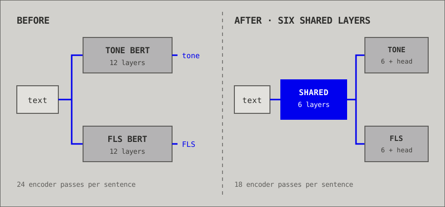
The models were finbert-tone and finbert-fls. Both use a 12-layer BERT architecture with a hidden size of 768 and 109,754,115 parameters each. Every sentence therefore passed through two full encoders before reaching two different classification heads.
Sharing Is Caring
At first I hoped the early layers might still be identical. Both models came from the same FinBERT base, and freezing lower pretrained layers is a common way to reduce the number of trainable parameters during fine-tuning. If those layers had been frozen, I could run them once and branch afterward.
I tried a quick check in the notebook. For one sentence, the models' layer-2 output summaries differed. But I hadn't switched the freshly loaded models to evaluation mode, so dropout could have contributed to that difference; I also hadn't compared their weights directly. The check didn't prove the early layers were different, and I couldn't assume they were identical either.
But it was too late: I decided to share them anyway.
The idea was not unprecedented. BERT and PALs and adapter modules show how much of a pretrained model can be shared across tasks when small task-specific parts are retained. Both would have required task data and another training run; I had neither the original data nor much time.
There are more sophisticated ways to merge already-fine-tuned models. Task Arithmetic combines their changes relative to a shared base, while TIES-Merging tries to resolve conflicting changes. I didn't test either. What I tried resembles model soups in one respect: averaging corresponding weights. But I averaged only the embeddings and lower encoder layers I wanted to share. For encoder layer , I took the corresponding weights from the tone and FLS models and averaged them element by element:
Here, and are the two sets of weights at layer , is their average, and is the number of encoder layers shared. The upper layers and classifiers stayed task-specific. This wasn't a novel merging method. It was partial weight averaging because it required no training data and took almost no time to implement. The question was how many layers I could share before the predictions moved too much.
How Many Layers Can Be Shared?
I tried sharing 2, 4, 6, 8, and 10 of the 12 layers. For the comparison, I used 500 unique passages from a financial-text classification dataset. I first sampled 600 rows without replacement, giving longer passages a higher chance of selection because they are more demanding inference cases. Some rows contained the same text, so I removed those duplicates and kept the first 500 distinct passages. This deliberately favors longer inputs rather than reproducing the dataset's natural length distribution. I didn't set a random seed, so the results are from one sample.
I cared less about reproducing exact logits or probabilities than about preserving the ordering of examples. Averaging weights can change the scale of a score without changing which sentence the model considers more positive or more forward-looking. What mattered was whether merging reversed which of two passages the original model scored as more positive or more forward-looking.
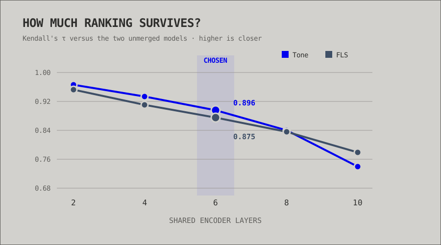
So I ranked texts primarily by positive-sentiment probability for tone and specific-FLS probability for FLS, then compared those rankings with the original models using Kendall's . For two rankings with no tied positions, count pairs that appear in the same order in both and pairs whose order is reversed:
That means the fraction of pairs that swapped order is . A of 1 means identical rankings; lower values mean more reversals. This measures agreement with the original models, not accuracy against ground-truth labels.
| Shared layers | Relative speedup | Tone | FLS | Size |
|---|---|---|---|---|
| 2 | 1.11× | 0.966 | 0.952 | 877.6 MB |
| 4 | 1.23× | 0.934 | 0.911 | 823.6 MB |
| 6 | 1.39× | 0.896 | 0.875 | 769.5 MB |
| 8 | 1.55× | 0.841 | 0.837 | 715.4 MB |
| 10 | 1.65× | 0.741 | 0.779 | 661.3 MB |
For the six-layer model, an FLS of 0.875 means roughly 94% of pairs of passages stayed in the same order as in the original model, while about 6% swapped places. Tone's 0.896 means about 5% of pairs swapped. These are comparisons with the original models' rankings, not claims that 87.5% or 89.6% of classifications were correct.
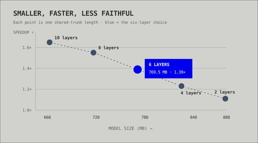
Sharing two layers barely changed the rankings. After six, the degradation became more noticeable; at ten, almost the entire encoder was being forced into the same weights despite the different fine-tuning tasks. I chose six shared layers: about 202 million combined parameters and a reported 1.39× speedup, with Kendall's of 0.896 for tone and 0.875 for FLS.
There is nothing special about six. If prediction fidelity mattered more, I might have stopped at two or four. For the capstone, it was a reasonable way to collapse a meaningful amount of computation without the two tasks immediately falling apart.
The speedup is directional rather than a controlled apples-to-apples benchmark: in this notebook, the original-model timer covers only the two forward passes, while the merged-model timer also includes tokenization and probability conversion. I would rerun both through the same timing boundary before making a stronger performance claim.
ONNX and Quantization
The shared model was faster, but it was still about 769 MB. The next steps were more conventional: export the merged PyTorch model to ONNX, optimize it, and dynamically quantize it to INT8.
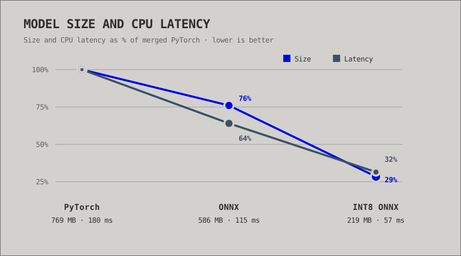
Here, the notebook timed the first 100 sampled texts on CPU, warming each model twice per text and excluding tokenization from all three measurements. From merged PyTorch to quantized ONNX, inference went from 180.37 to 56.91 ms per text and size from 769.34 to 219.32 MB: about 3.2× faster and 3.5× smaller. This was a larger improvement than sharing layers alone.
I didn't complete a controlled quality comparison for the quantized model, so the ONNX results here are size and latency results only.
I also replaced the Hugging Face tokenizer with a small JSON-backed implementation to reduce setup overhead, although I didn't benchmark that change.
A One-Off Hack
I needed these two models smaller and faster for a cloud deployment, and I couldn't retrain them. I worked backward from what I knew about how BERT's layers specialize and looked at similar techniques for clues. Both checkpoints came from the same FinBERT base, which gave me a reason to try something I wouldn't try with two arbitrary BERTs.
That was the fun part for me: drawing on existing interpretability research to think about what the layers might have learned instead of treating each model as a black box. I then developed a methodology to test that intuition on this particular pair.
It isn't the sort of thing I would have found in a blog post, because the use case was unusual and the approach isn't standard. Well, until now.
References
- Houlsby et al., 2019: Parameter-Efficient Transfer Learning for NLP
- Stickland and Murray, 2019: BERT and PALs
- Wortsman et al., 2022: Model Soups
- Ilharco et al., 2022: Editing Models with Task Arithmetic
- Yadav et al., 2023: TIES-Merging
- On the Transformation of Latent Space in Fine-Tuned NLP Models, 2022