The Geometric Median on Earth's Surface

Introduction

During a conversation, a classmate posed a seemingly straightforward question: "Where could we position our university, Minerva's Headquarters, to be at the least distance from all our classmates' residences?" This spot would be the most convenient for travel for everyone, regardless of where Minervans hailed from. Given that Minerva's student body comprises 180 individuals from around 60 countries, this query quickly evolved into an intriguing computational challenge.

At first, the solution appeared straightforward: simply find the average of everyone's locations. However, as I explored the project, I realized that the challenge was not merely pinpointing an average geographical midpoint. The task was to identify a location that minimizes the aggregate distance to all other points - a concept known as the geometric median.

It was only later that it struck me: contrary to my initial assumption, there is not a direct analytical formula to determine the two-dimensional geometric median. While solutions exist for one-dimensional medians and multi-dimensional geometric means, this problem remains elusive to a straightforward analytical approach.

Given the absence of traditional approaches to solving this puzzle, optimization techniques, known for their ability to refine solutions iteratively, emerged as the optimal choice.

The Problem Analyzed

Insert the definition of the geometric-median cost function using an L1 norm over distances between each point $x_i$ and candidate location $m$.

$$f(m) = \sum_{i=1}^{n} \left\lVert x_i - m \right\rVert$$

Clarify that this objective is non-differentiable where $x_i = m$, motivating numerical optimization rather than closed-form differentiation.

Provide the quadratic loss function used when optimizing for the arithmetic mean rather than the geometric median.

$$f(m) = \sum_{i=1}^{n} (x_i - m)^2$$

Note that this function is smooth and differentiable, allowing an analytical minimizer obtained by setting the derivative to zero.

Where (m) is the geometric median, (x_i) is some point on a two-dimensional plane, and there are (n) such points. Because of the absolute value in the first function, a discontinuity arises when (x_i - m = 0). Consequently, it is infeasible to directly differentiate this expression, equate it to zero, and discern an (m) value that minimizes the function. Various strategies exist to approximate this point. These methods might entail adjusting the cost function to resemble a differentiable one or deploying recursive algorithms that increasingly approximate the accurate solution. For this task, I employed a hill-climbing algorithm.

In our context, how do we find the distance (x_i - m)? Given that Earth approximates a sphere, the Haversine formula is applicable to determine the distance between any two points on its surface. This equation leverages longitudes and latitudes to calculate the angular distance between points. Once multiplied by Earth's radius, this angular distance yields the spatial separation on the Earth's surface in kilometers.

Insert the Haversine formula for great-circle distance between two latitude–longitude coordinates on a sphere.

$$a = \sin^2\!\left(\frac{\Delta \phi}{2}\right) + \cos(\phi_1)\cos(\phi_2)\sin^2\!\left(\frac{\Delta \lambda}{2}\right)$$ $$c = 2 \cdot \operatorname{atan2}(\sqrt{a}, \sqrt{1-a})$$ $$d = R \cdot c$$

Define (R) as Earth's radius and interpret (\Delta \phi) and (\Delta \lambda) as latitude and longitude differences in radians.

The Model

The given code implements a model called anealor_model that seeks to find the geometric median of a set of cities using the simulated annealing algorithm. In the context of this problem, the geometric median represents a point (city) that minimizes the sum of distances to all other cities.

Attributes:

• iterations (int): Represents the maximum number of times the simulated annealing process will iterate.
• alpha (float): Defines the cooling rate for the simulated annealing process.
• early_stopping_rounds (int): If there is no improvement after this many rounds, the process will stop early.

Functions:

• init: The constructor function initializes the class's attributes.
• haversine: Calculates the Haversine distance between two city coordinates.
• cost: Computes the total distance from a given city to a list of other cities.
• fixer: Adjusts coordinates to ensure they are within valid bounds for longitude and latitude.
• err_pc: Calculates the percentage error between the observed cost from a given point to the list of cities and the expected cost.
• annealer: The primary function that implements the simulated annealing algorithm.

How it finds the geometric median:

The simulated annealing algorithm starts with a random solution (a city with random coordinates), then iteratively makes small random changes to this solution and evaluates the resulting cost. The best solution found so far is retained, but worse solutions can also be accepted based on a probability related to the difference in cost and the current temperature.

By using a probabilistic acceptance criterion and gradually reducing the temperature, the algorithm balances exploration (trying out diverse solutions) and exploitation (refining the current best solution). This makes simulated annealing suitable for optimization problems like finding the geometric median, where the solution space can be rugged with multiple local minima.

Over time, as the temperature decreases, the model becomes less likely to accept worse solutions and starts to hone in on an optimal or near-optimal solution.

The result of this model will be the coordinates of a city that approximately represents the geometric median of the given cities.

Analysis

To determine the geometric median, the Geographic Midpoint Calculator was employed to determine the geometric median. This tool utilizes a recursive algorithm to approximate the geometric median with a precision of less than 0.00000002 radians error. In practical terms, this represents an incredibly small error of approximately 0.12 meters. However, the actual error might be slightly larger. This discrepancy arises because the assumption that the Earth is a perfect sphere may not be entirely accurate. When computing distances between distinct points, both methods pinpoint the geometric median hinge on this spherical assumption.

A percentage error is derived to assess our computed solution's accuracy. This is done by determining the difference between the cumulative Haversine distance (or cost) originating from our proposed solution and contrasting it with the cost from what is considered to be the near-optimal solution. This difference is then represented as a percentage of the cost from the near-optimal point.

For visualization purposes, the algorithm was executed for the full span of 5,000 iterations. In typical scenarios, the algorithm would halt its operation once the candidate point stabilizes and remains in a specific location for a prolonged period.

The temperature, which dictates the step size, is an essential aspect of the simulated annealing algorithm. As iterations progress, the temperature, and consequently the step size, diminish exponentially. Observations indicate that by the 500th iteration, most of the error reduction has already been achieved.

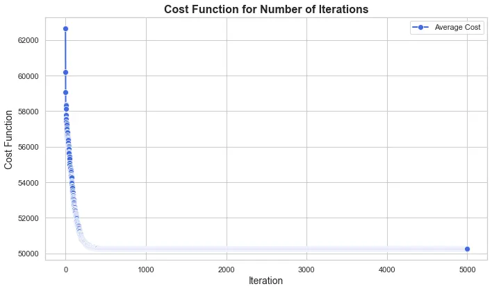
Fig. 1: Graphing the average cost function over number of iterations within the annealer.

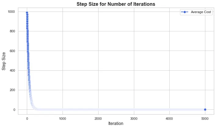
Fig. 2: Graphing the average step size over number of iterations within the annealer.

Considering the risk of candidate solutions becoming entrapped in local minima, conducting multiple runs of the experiments can yield more precise outcomes. However, directly averaging the x and y values of solution points might lead to skewed results, especially if there are extreme outliers in the x and y values. A more robust approach is to consider the median of the solutions. An even better strategy is to compute the average of the central 50th percentile of solutions to circumvent any skewness.

This said, the above functionality has not been directly incorporated into the code. For experiments with fewer than 10 replications, error is high. However, with a marginal increase beyond 10 repetitions, the results exhibit high precision. Notably, this heightened accuracy, while substantial, does not match up proportionally to the rise in computational costs, rendering the improvements relatively marginal.

Note that the graph is on a logarithmic scale.

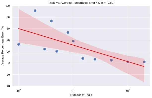
Fig. 3: Graphing the percentage error by number of trials the annealer was run.

The accuracy of the annealer displays a varied pattern depending on the number of cities considered. For the initial few cities, the error margin is quite pronounced. Interestingly, the annealer exhibits its peak performance when accounting for 4 to 13 cities, post which there is a modest uptick in error.

It is crucial to note that the accuracy is also influenced by the specific locations selected. The data set used to derive this analysis was generated randomly, indicating that different points might lead to different results.

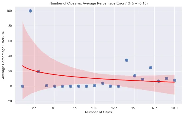
Fig. 4: Graphing the average error by the number of cities in the annealer process.

The algorithm's computational complexity is influenced mainly by cost calculation and the number of iterations.

Each iteration calculates the cost for a candidate solution by measuring its distance to every city in the list. Determining the distance between two cities is a constant-time operation, $O(1)$. But as this distance calculation is applied to all cities in the list, the cost computation per iteration scales linearly with the number of cities, making it $O(n)$. The algorithm undergoes $m$ iterations, where $m$ is a predefined constant.

Combining these components, the overall complexity of the algorithm is $O(m \times n)$. However, focusing on the algorithm's scaling with the number of cities, we can disregard the constant $m$ and conclude that the algorithm scales linearly with the number of cities: $O(n)$.

In essence, as the number of cities increases, the computation time for this algorithm will grow linearly. This can be observed in the approximately linear scaling in the following graph.

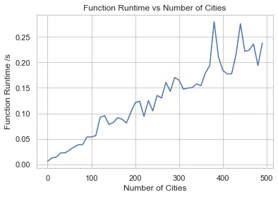
Fig. 5: Graphing the average runtime scaling of the program as the input increases.

7 Cities

A significant part of Minerva's allure is its global rotation system, where students experience diverse cultures in seven distinct cities worldwide. These cities include San Francisco, Buenos Aires, London, Berlin, Hyderabad, Seoul, and Taipei.

By applying our annealer algorithm, we attempt to identify the geometric median of these cities, which will essentially represent the most centrally located point relative to all seven cities. This point could conceptually serve as Minerva's "ideal" headquarters, provided we optimize for equidistant travel for students from each rotation city.

Predictions and Results

Anealer Model Prediction: Upon processing the coordinates of the seven rotation cities, the simulated annealing algorithm predicts the geometric median to be situated south of the Swedish island of Gotland. The predicted coordinates are (57.06, 17.44).

GeoMidpoint Result: A more precision-driven tool, GeoMidPoint Finder described earlier pegs the geometric median at coordinates (54.61, 14.43). This location is approximately 200 kilometers from the annealer's prediction, specifically south of Bornholm.

Conclusion

While both methods suggest locations within the Baltic Sea region as the central point, setting up an actual headquarters in the sea may not be the most feasible idea. Nevertheless, this exercise provides two insights. First, it offers a geographic representation of Minerva's expansive global rotation system. Second, it showcases the power and versatility of optimization techniques in addressing intricate challenges, particularly those devoid of clear-cut mathematical solutions.

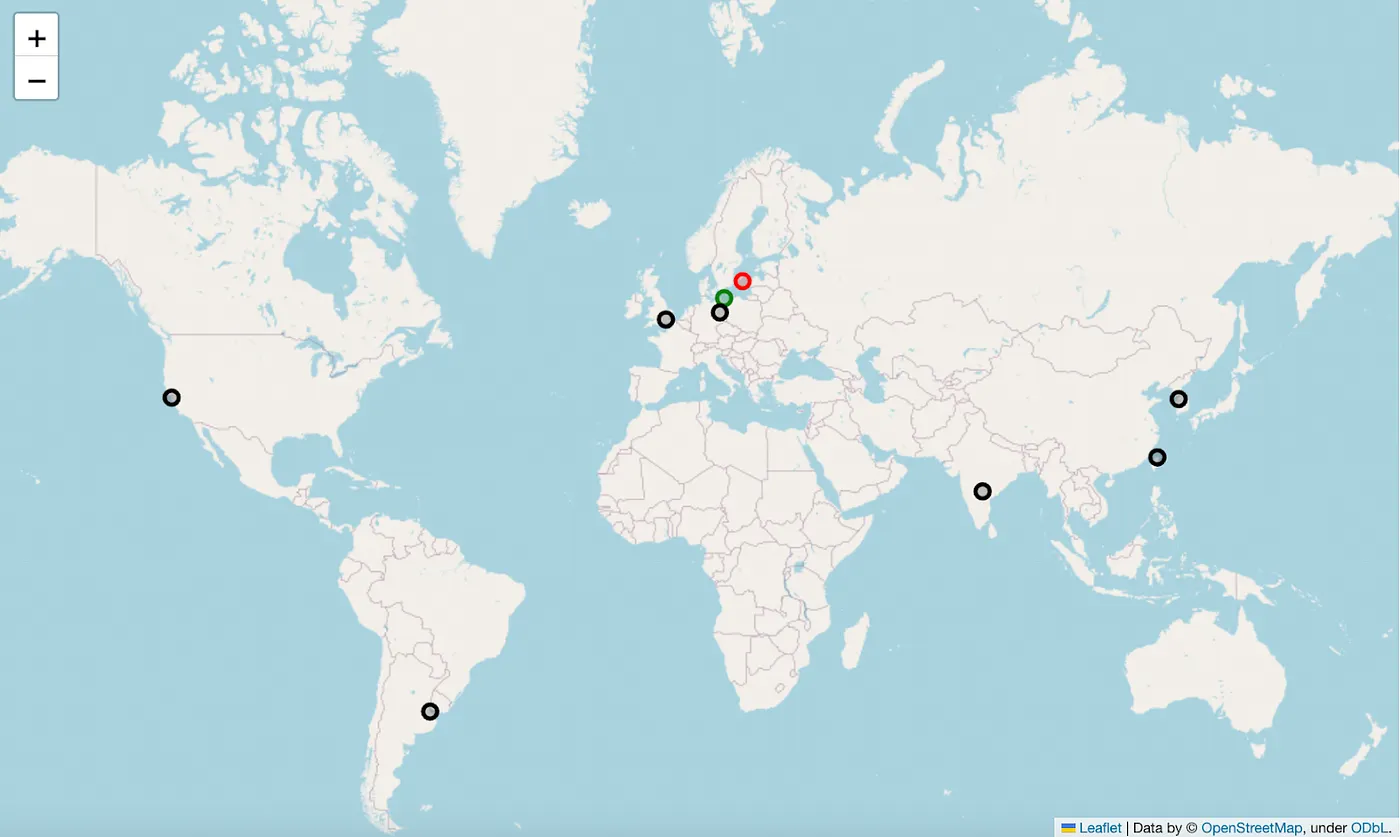
Fig. 6: Black: Minerva City, Green: Actual Geometric Median, Red: Predicted Geometric Median.

GIFs

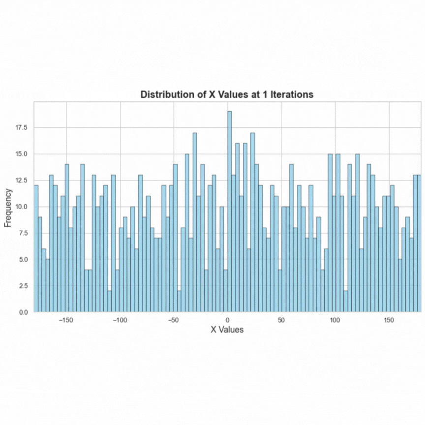
Fig. 7: Convergence of x values (latitude) to optima over the number of iterations.

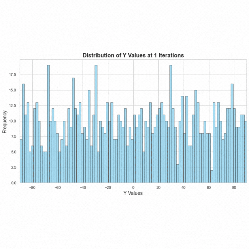
Fig. 8: Convergence of y values (longitude) to optima over the number of iterations.

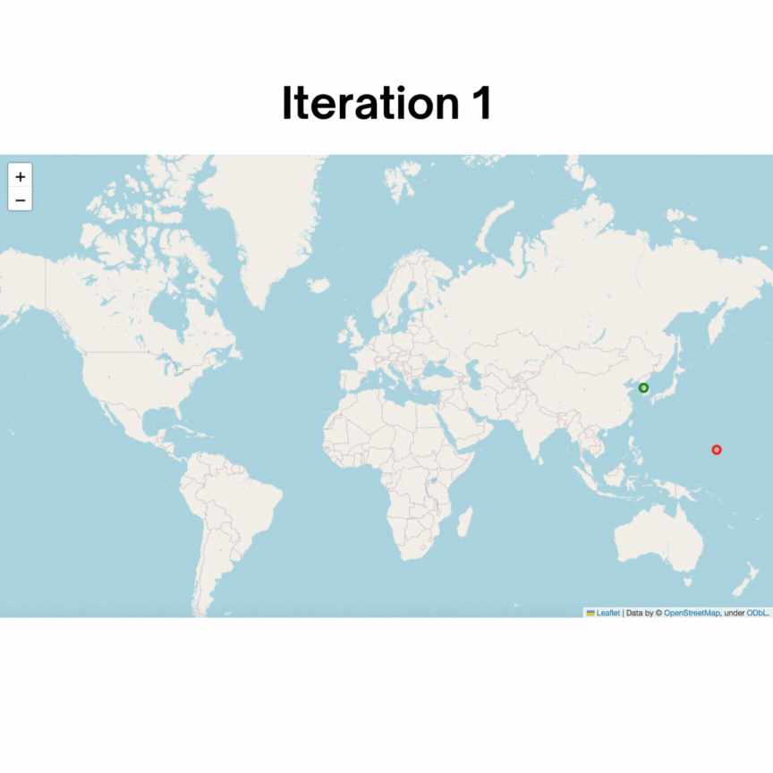
Fig. 9: Convergence to optima over the number of iterations.